Scripting with Python and JPype
|
The current User's Guide is very much a work in progress, any help would be greatly appreciated! |
Scripting openrocket with Python and JPype[edit]
Overview[edit]
The ability to script OpenRocket and enhance it with user written code is an often discussed topic among the OpenRocket community. This article demonstrates one approach to the problem. Using Python and the JPype library it is possible to write external scripts which run outside of OpenRocket, but make use of OpenRocket much like any other python library.
This approach provides a very rapid development environment for optimizing rocket designs, enhancing and exploring the simulation. It is also probably the best approach if you are interested in making use of OpenRocket as part of something larger. An important advantage to this approach over something like embedded Jython scripting is that you have full access to all the python ecosystem, crucially numpy, scipy, matplotlib and other cpython only libraries. However, because scripts require external software they can not be integrated into a stand-alone OpenRocket distribution. Nevertheless, they do provide a nice way to prototype new OpenRocket features.
Requirements[edit]
To run the following examples you will need Python 3.6 or later and OpenRocket-15.03.jar. The numpy, scipy, matplotlib libraries are required (these usually come together). These scripts all make use of a python package orhelper (below).
Orhelper[edit]
This is a fairly lightweight module which has been written for these examples to take care of some of the more cumbersome aspects of scripting OpenRocket with jpype.
At the time of writing the orhelper module contains:
- a class OpenRocketInstance which handles starting up a JVM and a working openrocket instance. It is equipped with __enter__ and __exit__ methods and is intended to be called using the with statement. This is to ensure that no matter what happens within that context, the JVM will always properly shutdown and you will get useful (hopefully) exception information.
- a class Helper which simply contains a bunch of useful helper functions and wrappers for using openrocket via jpype. These are intended to take care of some of the more cumbersome aspects of calling methods, or provide more 'pythonic' data structures for general use. The whole net.sf.openrocket namespace is available as the orp property of this class.
- an AbstractSimulationListener class. This is essentially a python version of the openrocket.simulation.listerners class of the same name. You can extend this class to make your own python simulation listeners and receive callbacks from the openrocket simulation.
- there is also a little wrapper class in there, JIterator which is for using java iterators as if they are python iterators.
Example 1 (simple_plot.py)[edit]
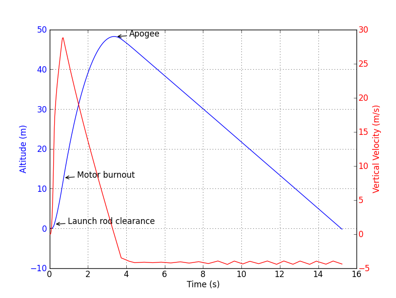
This is a simple example for plotting the flight of a rocket using matplotlib. A plot of altitude and vertical velocity vs time is generated, with annotations for various events much like the default plot in openrocket.
In this example all the interaction with OpenRocket is done through various Orhelper methods. The orhelper.Helper class will from now on be referred to as orh.
First, we startup an openrocket instance inside the protected 'with' environment. Be sure to change the name of the OpenRocket .jar file accordingly. We then load up an openrocket document, I am using the 'simple model rocket example' here. We then grab a simulation object out of this file. This file has multiple simulations set up, we just get the first one. We then run the simulation. We now need to get the data out of the simulation. This is done with the orh.get_timeseries method. This returns dictionary of timeseries data (as numpy arrays) from a simulation given a sequence of variable types. For adding annotations to the plot, we need to get a dictionary containing all the flight events. This is done with orh.get_events.
The rest of the code is standard matplotlib stuff -- check their documentation if you are not familiar. A couple of the inline functions though are worthy of further explanation. I wanted to have the axis labels and tick marks the same colour as the lines. Matplotlib doesn't have a built in way to change all the tickmarks, but that is easily done with the in line function change_color. Also, because get_events only gives us time information we need to extract the corresponding array index to put the annotations in the correct place. This done with the index_at function which in turn makes use of the numpy argmin function.
Example 2 (lazy.py)[edit]
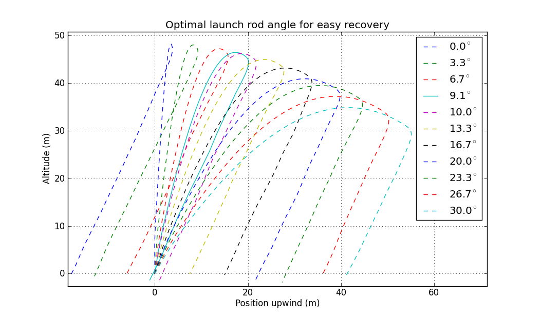
The purpose of this example is to show how a simulation can be modified and demonstrate the use of scipy's numerical methods. The toy problem we are attacking is the one of the rocketeer of maximum laziness who does not want to walk from the launch site to collect the rocket and would prefer if it flew exactly back of its own accord. We assume the rocket is flying upwind and optimise the launch rod angle accordingly. We want to plot a family of curves for a few different angles and highlight the optimised angle.
The structure of the program and initial lines for loading the model rocket are the same as in the previous example. In this example, we need to define a function for varying the launch angle before simulating the flight. This requires us to get the simulation options out of the simulation using the getOptions() method and we can then set the angle inside the SimulationOptions object. For the uninitiated, in OpenRocket simulation.SimulationOptions basically contains all the settings found in the simulation edit window. When the simulation is started these options are used to make a simulation.SimulationConditions object. After running the simulation we are interested in the ALTITUDE and POSITION_X variables. One option would be to just retrieve the final values with orh.get_final_values, however for reasons that will shortly become clear we have retrieved the whole time series.
For running an optimisation method, we need some function which is zero at the optimum point. This is not quite as simple as just getting the final upwind distance because the simulation stepper will usually slightly overshoot and calculate a final point with a negative altitude. We also want to exclude the launch. There are more elaborate ways this could be done --- here for simplicity we just slice out the last half of the data, find the index with the smallest absolute altitude and return the corresponding upwind distance. We can then go ahead and pass this to our optimisation method, giving some initial guess (40 deg) to start with. Scipy has a wide range of optimisation methods with a rich heritage, in our case we just choose the basic fmin which uses the downhill simplex algorithm.
In this example we want to plot a family of curves as well so we generate a range of 10 launch angles with np.linspace and add our optimal angle. We then run the simulations, making a dictionary of all the timeseries data with an 'Angle' key. We then go ahead and plot this, using a solid line style for the optimal curve and dashed lines for the others.
Example 3 (monte_carlo.py)[edit]
As every student of introductory physics knows, presenting just a number as the result of a calculation is not really sufficient -- we also need to know the uncertainty to make it meaningful. The purpose of this example is to demonstrate a simple monte carlo method where multiple simulations are run with various parameters perturbed to determine an overall uncertainty for the landing location in terms of range and bearing from the launch site. This example also demonstrates the use of simulation listeners implemented in python. Openrocket simulation listeners are covered in section 9 of the users guide.
The structure of this script is slightly different from the previous examples. First consider how we get the landing range and bearing information. We do this by defining a new simulation listener LandingPoint which extends orhelper.AbstractSimulationListener. We define an endSimulation method which grabs the lanuch site WorldCoordinate (from SimulationConditions) and the rocket position (from SimulationStatus) to calculate the range and bearing. These are saved as LandingPoint instance variables.
Multiple LandingPoint objects are stored in a LandingPointList, which is like a regular list except can populate itself with landing points by running multiple openrocket simulations. Various parameters are set by choosing from a gaussian distribution with given mean and standard deviation (pythons random.gauss method). The code for running the simulations has mostly been discussed earlier, and the same example rocket is used although in my case I turned up the wind and turbulance somewhat and switched to a spherical earth computation method. One aspect that is new is the modification of the rocket model. A rocketcomponent.Rocket object can be obtained from the simulation options. This is the root of a tree type data structure containing all the rocket components. Our orh.Helper class has a method for finding components in the tree given their names. We use this to obtain the nose cone and body tube components and override their masses with perturbed values. Running the simulation is again done using orh.runsimulation, except in this case we pass in a sequence of listener objects to use. To increase the variability still we pass in a AirStart listener with randomly set start altitude. This listener is a python copy of the example supplied with openrocket.
Finally, when run the main function of the script makes a new LandingPointList, populates it and then uses the print_stats method to show the final landing statistics, something like:
Rocket landing zone 3833.57 m +- 1116.91 m bearing -89.98 deg +- 0.0713 deg from launch site. Based on 20 simulations.
Note that it might take a minute or two to run all those simulations.

